

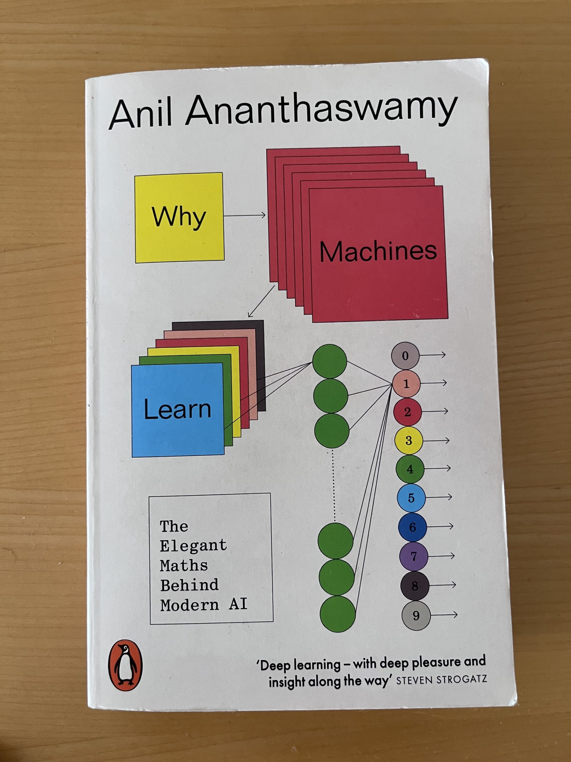
The Machine Learning
In 1958 Frank Rosenblat invented the perceptron. It never lived up to the hype.
Understanding how machines learn demands embracing equations and concepts from at least four major fields of mathematics: linear algebra, calculus, probability and statistics, and optimization theory.
Desperately Seeking Patterns
What are patterns in data?
Y=wlxl + w2x2
The relationship between y, xl, and x2 is defined by constants wl and w2. These constants are called the coefficients, or weights.
If there’s a way to algorithmically figure out the weights, then the algorithm is “learning” the weights.
The perceptron0’s roots lie in a 1943 paper. Warren McCulloch was an American neurophysiologist trained in philosophy, psychology, and medicine. He was thinking about brain as computational device. Together with Walter Pitts proposed a simple model of a biological neuron. Turned it into a simple computational model, an artificial neuron. They showed how using it you could implement certain basic Boolean logical operations such as AND, OR, NOT.
Perceptron could learn weights from data.
Donald Hebb named the process (neurons that fire together wire together) Hebbian learning.
Much of machine learning comes down to minimizing prediction error.
Is identifying correlations the same thing as thinking and reasoning.
We Are All Just Numbers Here …
Sir William Rowan Hamilton created the algebra for manipulating quaternions, and to do that he developed some mathematical ideas that have become central to machine learning. In particular, he introduced the terms scalar and vector.
A scalar quantity is a stand-along number. If we have two pieces of information, can be represented by a vector. It has length and a direction.
It was already Isaac Newton who was using geometric way of thinking about vector-like entities such as acceleration and force.
Gottfried Wilhelm Leibniz (1646-1716) wrote to Christiaan Huygens that he believed that he found a new way to represent figures and even machines and movements by characters, as algebra represents numbers or magnitudes.
Vector analysis doesn’t have to be geometric. It can come down to manipulating numbers written in a certain format. And in fact, for machine learning, that’s how we need to think about vectors.
One can multiply a vector by a scalar. A unit vector is simply a vector with a magnitude of 1. Another important operation with vectors is something called the dot product. One important thing the dot product tells us about two vectors is whether they are at right angles, or orthogonal, to each other. If they are at right angles, the cosine of (90) equals zero.
A set of weights (w1, w2) is nothing but a vector w. but what exactly does w represents.
Each data point is given by (x1, x2). The weighted sum (w1x1 + w2x2) is the same as the dot product of the vector representing, the data point with the weight vector.
It’s clear that the dot product of each vector with w is telling you something about that vector: its distance from the hyperplane and whether it’s to one side of it.
Data points are just arrays of numbers, each array with two elements. The weight vector is similarly another array of two numbers. Finding the dot product is a matter of manipulating these arrays. More generically, these arrays are called matrices.
Flipping the matrix on its side is called taking the transpose of a matrix. Taking the transpose is a key aspect of calculating the dot product between two column matrices. The transpose of A is written as AT. The dot product A.B is written as ATB or BTA.
The task of a perceptron is to learn the weight vector, give a set of input data vectors, such that the weight vector represents a hyperplane that separates the data into two clusters. Once it has learned the weight vector, and then is given a new data point to classify.
Minsky and Papert proved that single layer of perceptrons cannot solve such problems as separating two triangles (0,1) and (1,0) with circles (0,0) and (1,1). It is called XOR problem.
In 1986, David E. Rumelhart, Geoffrey E. Hinton and Ronald J. Williams published a pathbreaking paper on an algorithm called backpropagation. The algorithm which showed how to train multi-layer perceptrons, relies on calculus and optimization theory.
The Bottom of the Bowl
It was the autumn of 1959, Bernard Widrow was in his office at Stanford when a graduate student named Marcian Ted Hoff came looking for him. During that discussion, the two invented what came to be called the least mean squares (LMS) algorithm, which has turned out to be one of the most influential algorithms in machine learning.
The term “artificial intelligence” is credited to John McCarthy, a mathematics professor at Dartmouth College.
In 1847 Baron Augustin-Louis Cauchy proposed the method of steepest descent. The steepest route is also the shortest path down. You do that by evaluating the slope, or the gradient. One way to find the slope of a curve is to draw a tangent to the curve at the point of interest.
Differential calculus is a branch of calculus that lets us calculate the slope of a continuous function. The slope in general is zero at the minimum of a function.
We are now equipped to understand the method of steepest descent, also known as the method of gradient descent.
These seemingly disparate fields of mathematics – vectors, matrices, linear algebra, calculus, probability and statistics, and optimization theory – will all come together as we make sense of why machines learn.
In the field of signal processing, a filter is something that that takes a input signal, processes it, and produces an output signal that has certain desired properties.
How should we calculate the average error? Negative and positive errors can negate each other. We could add the absolute value of the errors and take the average; this is called the mean absolute error (MAE). But the match folk prefer to take the average of the square of the error terms and call it a mean squared error (MSE). If you want your error estimate to punish the extreme outliners, then the MSE does that better than the MAE.
When Hoff walked into Widrow’s office they came up with an idea that they could get a stochastic gradient, a very crude gradient, algebraically – without differentiating anything, without averaging anything, and without squaring anything. The adaptive neutrons by Widrow and Hoff. The algorithm uses input and the desired output to adjust its weights and generate the correct output.
The gradient is simply a vector in which each element is the partial derivative of the mean squared error, with respect to each weights.
Widrow and Hoff decided that instead of calculating the entire gradient, they calculated only an estimate of it. The estimate would be based on just one data point. For each input, you calculate the error and use that to update the weights. It came to be called the least mean squares (LMS) algorithm.
Every deep neural network today uses some form of gradient descent for training.
The LMS algorithm is the foundation of backdrop. And backdrop is the foundation of AI.
In All Probability
Probability deals with reasoning in the presence of uncertainty.
Two ways of thinking about probability: frequentist and Bayesian. The frequentist notion of the probability of occurrence of an event is simply to divide the number of times the event occurs by the total number of trials. Bayes’s theorem gives us a way to draw conclusions, with mathematical rigor, amid uncertainty.
The theorem allows us to calculate the probability of a hypothesis H being true, given the evidence E. This is written as P(H/E): the probability of H given E.
P(H/E)= P (H) x (PE/H)/ P(E)
P(H): The prior probability.
P(E/H). The probability of the evidence given the hypothesis.
P (E): The probability of evidence – all the possible ways of evidence.
The final number is called the posterior probability. It’s the prior probability updated given the evidence.
Most machine learning is inherently probabilistic, even if the algorithm is not explicitly designed to be.
Bernoulli distribution is example of a probability distribution.
In distribution the important statistical parameters are the variance, the standard deviation, the expected value. The standard deviation is defined as the square root of the variance. The variance and standard deviation are telling you something about the spread of values away from the mean.
Whether it’s probability mass function for a discrete random variable or a probability density function for a continuous random variable, some well-known and analytically well-understood function, with characteristic parameters, can be used to describe the probability distribution.
Two important approaches. First is MLE – maximum likelihood estimation. The second is MAP – maximum of posterior estimation.
One of the first large-scale demonstrations of using Bayesian reasoning for machine learning was due to two statisticians, Frederick Mosteller and David Wallace.
ML algorithm are basically trying to get at the best possible approximation of the underlying distribution from a sampling of data.
A classifier, with the assumption of mutually independent features, is called a naïve Bayes or, somewhat pejoratively, an idiot Bays classifier.
The task of many ML algorithms is to estimate the distribution, implicitly or explicitly, as well as possible and then use that to make predictions about new data.
Any algorithm that figures out how to separate one cluster of data points from another by identifying a boundary between them is doing discriminative learning. The latest algorithm is called the nearest neighbor (NN) algorithm.
Birds of a Feather
A Voronoi cell (after Georgy Voronoi) is a cell in which any point inside the cell is closer to the defined point in that cell than any defined point in other cells.
In computer science, similarity has to do with the distance of one data point from another in some hyperdimensional space.
The nearest neighbor rule algorithm was created by Thomas Cover and Peter Hart.
The nearest neighbor algorithm, in its simplest form, essentially plots that new data point and calculates its distance to each data point in the initial dataset, which can be thought of as the training data.
Perhaps the most important feature of the k-NN algorithm is that it’s a so-called nonparametric model. A nonparametric model has no fixed number of parameters. That is also his problem, since the computational requirements grow with dataset growth.
As the number of dimensions tends to infinity, the volume of the unit sphere tends to zero.
PCA – principal component analysis is a powerful technique to reduce the data to some tractable number of lower dimensions, allowing an ML algorithm to do its magic.
There’s Magic in Them Matrices
Working with high-dimensional data can drain computational resources.
A matrix is a rectangular array of numbers. Machine learning comes down to manipulating vectors and matrices.
Multiplying a vector by a matrix can transform the vector by changing not just its magnitude and orientation, but the very dimensionality of the space it inhabits.
Special orientations, or vectors, associated with a square matrix are called eigenvectors. Corresponding to each eigenvector is an eigenvalue.
The Iris dataset is a bit of a marvel as a dialectic tool for modern machine learning. It was published in a 1936.
The Great Kernel Rope Trick
Vladimir Vapnik created a method that is systematic method for finding the best possible separating hyperplane that minimizes errors when classifying new data points.
Vapnik requested that Boser push data that was linearly inseparable in lower dimensions into some higher dimensions. The algorithm needs to simultaneously do two things: create new features such that the data can be mapped into some higher-dimensional space, and avoid having to perform dot products in that new space and still be able to find the separating hyperplane.
The problem of constrained optimization can be thought of as finding the extrema of the so-called Lagrange function.
In a infinite-dimensional space, you can always find a separating hyperplane.
John Hopfield. He described a novel way of constructing neural networks that could be trained to store memories. These networks were called Hopfield networks.
The method of using kernel function (K function) to compute dot products in some higher-dimensional space, without ever morphing each lower-dimensional vector into its monstrously large counterpart, is called the kernel trick.
The combination of Vapnik0s 1964 optimal margin classifier and the kernel trick proved incredibly powerful.
Vapnik and Corinna Cortes developed what they called a soft-margin classifier. They called their algorithm support vector network. Berhard Scholkopf renamed it into support vector machine.
With a Little Help from Physics
John Hopfield looked at transfer RNA, or tRNA, molecules that recognize the correct amino acids and bring them to the site of protein synthesis in cells. If you could describe the equation of how neural activity propagated from one neuron to another you had a dynamic system.
Our brains are somehow able to use a fragment of the original experience to bring into conscious awareness an entire stored memory. That’s associative memory.
In early 1920s, Wilhem Lenz and Ernst Ising developed Ising model. The model described how any given spin (magnetic moments) state is influenced only by its immediate neighbors.
Hopfield defined the stored memory state as low-energy state. This state was characterized by the strengths of the connections, or the weights, between the neurons.
In the 1970s, researchers were beginning to probe how to train multi-layer networks. The outline of an algorithm that would soon be called backpropagation, or backdrop, was taking shape.
Neurons that fire together wire together. Here, wiring together means changing the weights between two neurons such that the activity of the neurons is reinforced. Choosing the weights to accomplish this is called Hebbian learning.
Hopfield networks are what are called one-shot learners. Given one instance of data, the network can memorize it.
1986 the first detailed explanation of backpropagation algorithm was published by George Cybenko.
Theorem: If a Hopfield network in a stable state is perturbed, then it will dynamically transition through a series of states until it reaches and settles into a stable state that represents an energy minimum.
Whether or not a neuron flips depends on the weights and the outputs of all the other neurons to which it’s connected. If the field of a neuron has the opposite sign to its current state, the neuron flips; otherwise, it doesn’t.
The Man Who Set Back Deep Learning (Not Really)
Cybenko’s proof showed that a neural network with just one hidden layer, given enough neurons, can approximate any function, meaning it can turn an input into any desired output. The theorem is called the universal approximation theorem,
If a network requires more than two weight matrices (one for the output layer and one for each hidden layer), then it’s called a deep neural network: the greater the number of hidden layer, the deeper the network.
A training algorithm, such as backpropagation, will find the weights and biases using training data.
Functions are vectors in an infinite-dimensional space.
The Algorithm that Put Paid to a Persistent Myth
While his friend was exploring how memories are stored, Geoffrey Hinton became interested in how brains learn; he wanted to understand the mind. He was deeply influenced by Donald Hebb’s book The Organization of Behavior.
Rosenblatt had introduced the idea of backpropagation as a means for training multi-layer networks, but hadn’t figured out exactly how to do it.
In the early 1980s, Rumelhart, Hinton and Williams developed their algorithm.
Update the weight and bias, reevaluate the loss, and keep doing this until the loss falls below an acceptable limit; then stop.
There’s a very important and interesting question about whether biological brains do backpropagation. It’s very likely that our brain are implementing a different learning algorithm.
Training eventually comes down to this: provide the network with some set of inputs, figure out what expected output should be, calculate the loss, calculate the gradient of the loss, update the weight/biases, rinse and repeat.
The ability to create useful new features distinguishes back-propagation from earlier, simpler methods such as the perceptron-convergence procedure.
The Eyes of a Machine
David Hubel and Torsten Wiesel were the co-founders of the Department of Neurobiology at Harvard. Hubel’s invention of a tungsten electrode to record the electrical activity of single neurons, or units, in the brain, happened in 1957.
The visual field is the region in front of us that our eyes are sensitive to at any instant. The receptive field refers to the portion of the visual field that triggers a single neuron.
In 1975, Kunihiko Fukushima announced the first real neural network-based image recognition system of considerable complexity.
Yann LeCun used convolutional neural network (CNN) that uses the backpropagation algorithm. Instead of backpropagation gradients, or calculating all the partial derivatives using the chain rule, LeCun’s algorithm backpropagated ‘virtual target values’ for each hidden unit.
The debate if our cognitive capabilities are mainly innate (Chomsky’s position) or whether they are the outcome of learning that happens during development (Piager’s position).
In 1989 Krizhevsky, Sutskever, and Hinton build AlexNet.
Even before the advent of AlexNet, Hinton and a graduate student named Volodymyr Mnih understood the usefulness of GPUs. The large network required GPUs, by then, these came equipped with the software called CUDA. Mnih wrote another package atop CUDA, called CUDAMat.
Terra Incognita
Our task is to train an ML model to perform regression, to find a curve that fits the training data in a way that will allow the model to generalize well to unseen data.
How does one choose the correct level of complexity of the model? This leads to the two competing forces at work here. One is called bias: The simpler the model, the greater the bias. The other one is called variance: The more complex the model, the greater the variance. High bias leads to underfitting. High variance leads to overfitting. A job of an ML engineer is to find the sweet spot.
With deep neural networks this trade off was not that important any more.
LLM learns the statistical structure of language.
Deep neural networks, despite being over-parameterized, generalize well.
Epilogue
Theory of mind is a cognitive ability humans have that allows us to make inferences about someone else’s beliefs or state of mind using only external behavioral cues.
Brains are vastly more capable in certain ways, but LLMs are so much faster at certain tasks.
Are Transformers All We Need?
Attention Is All You Need was a 2017 paper by Ashish Vaswani. Transformers are the architecture that relied solely on something called attention for translating text from one language to another.
The decoder-only transformer: representing data as vectors, estimating probability distributions, embedding data in vector spaces, manipulating matrices and vectors, the universal approximation theorem, training a neural network using gradient descent and the backpropagation algorithm, and even self-supervised learning.
In the figure of the layout of the transformer, you’ll see something called Positional Embedding added to the input embedding, before the data enters the transformer layer. This is because words have meanings in part because of their position.
The first computation that happens in the attention mechanism is that each word or more precisely its embedding, gets associated with a set of three vectors: query – q, key – k, value – v.
The transformer takes the incoming embedding vectors (x1, x2, …. , xn) and transform each vector using the learned Query Wq, Key Wk, Value Wv, weight matrices to produce the matrices Q, K, V. The final formula for masked self-attention in matrix notation is:
Masked self-attention (Q, K, V) = softmax (QKt/√dk + M)V.


